Train your model
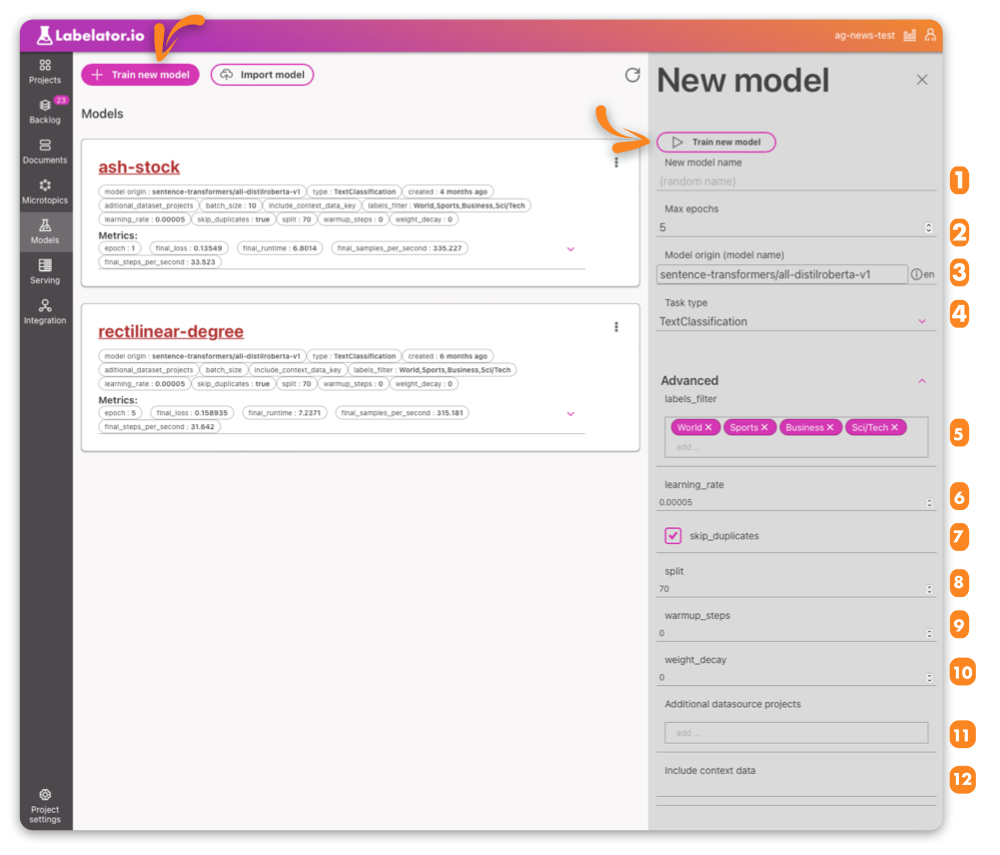
To train a new model, go to Models/Train new model. There, you can name your model and set up basic training parameters such as the number of epochs, the source model to fine-tune, and the general task type.
Understanding the training setup
Basic training settings
1. Name of the model
If you wish to name the model, you can do so here. If you do not provide a name, a unique random name will be generated for you.
2. Max epochs
The maximum number of epochs is the number of iterations over the training set that the model will undergo. The appropriate value for this parameter can vary.
Early stopping
If during the training process we determined, that further training is not beneficial, the training will be stopped before the number of epochs is reached (hence the parameter is named "Max epochs"). This is evaluated on the evaluation part of the dataset. The amount of data used for evaluation is determined by the split parameter (in advanced parameters section).
3. Model origin
In general, we do not train a model "from scratch" as this would require a large amount of data. Instead, we "fine-tune" an existing model that has been trained on a general language understanding task such as masked language modeling (MLM), where a randomly selected word is hidden from the model and its task is to predict the word from the context. While this task is useful for improving the model's general language understanding, we still need to fine-tune the model for our downstream task, which is determined by the project type.
By default, we use the sentence similarity model preset in the project for fine-tuning, but you can choose any model that you have trained in the past or any PyTorch transformer model from the Hugging Face hub. You can even import and fine-tune your own proprietary model.
4.Task type
While the task type is predetermined in the project settings, you can change it here. Training text similarity in a classification model can often be beneficial, especially when applied to the project to further improve similarity matching for labeling.
Advanced training settings
5. Labels filter
You can exclude some labels from training. Especially if you don't have enough sample data for them, excluding them from training might be beneficial. You can train a model that will include them later.
6. Learning rate
The learning rate determines the speed at which the model learns from the training data. If the learning rate is too high, the model may skip over the optimal solution and converge on a suboptimal one. On the other hand, if the learning rate is too low, the model may take a long time to converge on the optimal solution.
If you choose a smaller learning rate, it is advised that you also increase the number of epochs (especially if you are fine-tuning a model that has not been trained on this classification task yet).
If your learning rate is too big, the training might even become unstable. Your model won't be able to train, or will simply start to predict the most likely label for any prompt. This can often be fixed by decreasing the learning rate. You can see this also on the loss curve (it will suddenly jump to higher values and will stay there).
7. Skip duplicates
Having too many duplicate documents in your training set might hurt the training, therefore this parameter is turned on by default. However, finding the duplicates consumes resources and time, and if you know that you don't have them in your dataset, you might disable this option.
8. Split
Split is defined as the percentage of data that is being used for training.
The training/evaluation split is the process of dividing the data used for training a machine learning model into two separate sets: a training set and an evaluation set. The training set is used to train the model, while the evaluation set is used to evaluate the model's performance on new data. This helps ensure that the model is able to generalize to new data, not just memorize the training data.
This is also important for Early stopping, as the evaluation part of the dataset is used to determine whether we are still learning, or just memorizing the correct answers.
9. Warmup steps
Setting up warmup steps we gradually increase the learning rate (which determines the speed at which the model learns from the training data) over the first few training steps. This helps the model "warm up" and get used to the training process before diving into more challenging tasks. By starting with a higher learning rate and gradually decreasing it over time, the model can avoid getting stuck in suboptimal solutions and converge on a better one more quickly.
10. Weight decay
Weight decay is a technique used to regularize a model by reducing the weights of certain parameters that have large magnitudes. In machine learning, each piece of data (called a "parameter") has a weight that determines how important it is to the model's predictions. Sometimes, certain parameters can have very large weights, which can make the model hard to train and prone to overfitting (performing poorly on new data). Weight decay reduces the weights of these large parameters to make the model easier to train and more generalizable to new data.
11. Additional data source projects
You can combine data from multiple projects as long as they have the same labels or there is at least an overlap.
This is useful if you have a general dataset available and want to combine it with the current project.
12. Include context data
In general, the model only uses the main text to predict the correct label. However, sometimes there is additional metadata that can help the model make better predictions. You can include this data in the training by setting the metadata parameter name.
Currently, you can add only one additional parameter.
Understanding the training evaluation
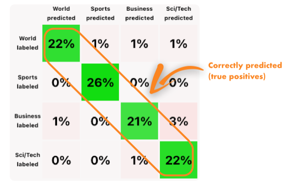
Confusion matrix
In a confusion matrix, the true positives are placed on the diagonal axis going from the top-left corner to the bottom right. Here, we can see the percentage of the data that was labeled as class N and also predicted as class N. In the Nth row, we can see the percentages of all the other classes that have been predicted.
In general, we want to see the most amount of data in the true positive zone. If we see that for a particular class, there is a higher percentage of data predicted as a different class than it was labeled (i.e., the model confused one class for another more often), that is something we can focus on.
To address this issue, we can go over the data that has been predicted and labeled as such (see filtering data). There are three possible scenarios:
Some data has been mislabeled. The model is correctly predicting the right label, but the document has not been correctly labeled. In this case, we can fix the labels to achieve better evaluation results.
The labels are correct, but the predictions are not. In this case, we might want to provide more similar examples to those that were incorrectly predicted. We can also look at similar documents, as they might be incorrectly labeled and therefore the model was given wrong training data.
We have enough data, all labels for this and similar data are correct, yet the model is giving us wrong predictions. In this case, it is possible that the model simply can't detect the correct class from the text. Sometimes, external knowledge is needed to get the right answer. If possible, consider adding this as metadata to the documents. Also, check whether the labels for this kind of data are consistent.
Evaluation metrics
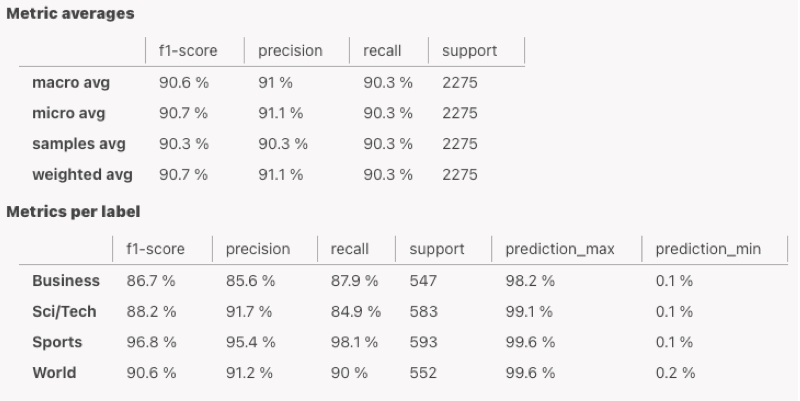
Precision: Precision is a measure of a classifier's exactness. It is calculated as the number of true positives divided by the sum of the true positives and false positives. A high precision score indicates that the classifier rarely labels a sample as positive when it is actually negative.
Recall: Recall is a measure of a classifier's completeness. It is calculated as the number of true positives divided by the sum of the true positives and false negatives. A high recall score indicates that the classifier correctly identified most of the positive samples.
F1 score: The F1 score is a measure of a classifier's performance, calculated as the harmonic mean of precision and recall. It is used to balance precision and recall, as it assigns a higher weight to lower values. A high F1 score indicates that the classifier has a good balance of precision and recall.
Support: The number of documents used to calculate this metric
Macro average: Macro average is a method of averaging precision, recall, and other metrics across classes. It calculates the metric for each class and takes the unweighted mean of these values. This method does not take label imbalance into account, meaning that it gives equal weight to all classes regardless of the number of samples they contain.
Sample average: Sample average is a method of averaging precision, recall, and other metrics across classes. It calculates the metric for each sample and takes the mean of these values. This method gives more weight to samples that are in classes with a larger number of samples.
Weighted average: Weighted average is a method of averaging precision, recall, and other metrics across classes. It calculates the metric for each class, takes the average of these values, and weights the result by the support (the number of true instances for each label). This method gives more weight to classes with a larger number of samples and to classes that are more important.
Micro average: Micro average is a method of averaging precision, recall, and other metrics across classes. It calculates the metric for all samples by considering each element of the label indicator matrix as a label. This method gives more weight to samples that are in classes with a larger number of samples.
Understanding training metrics
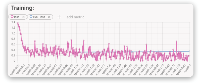
Training loss and evaluation loss are important metrics to monitor during training. Loss represents the amount of error made by the model during training. The model tries to minimize its loss, which means minimizing the number of errors it makes.
Ideally, training loss has a decreasing trend and the same should be true for evaluation loss. However, at some point, evaluation loss may start to grow. This is usually a sign of overfitting, which means that the model is effectively not learning to understand the problem, but rather remembering the correct answers. As a result, it continues to improve its training loss, but performs worse during evaluation (which tests its performance on previously unseen data).
Another sign to look for is when training loss suddenly jumps to high values and stops improving. This might be a sign of unstable training. In this case, it can be useful to change the learning rate or weight decayto stabilize the training.